

Today, we invite guest blogger Rune Thygesen of Reelight to discuss designing a power generation source for bicycle safety lights using simulation.
At Reelight, we are developing an affordable bicycle safety light that is extremely easy for the end user to install. Along with a stronger and more flexible mounting system, we needed to develop a new power generation platform. Using simulation-based design, we created a power platform that is easy to use and quick to install.
Designing Bicycle Safety Lights with the Rider in Mind
If you have been to Copenhagen in Denmark, you have probably noticed the hub-mounted flashing lights that are on the majority of bikes. Urban commuters prefer these lights because they’re already attached to the bike, so they can’t be forgotten at home. The bicycle lights are usually sold together with the bikes, thus mounted by the local bike store.
With our research, we aimed to create a light tailored for the consumer by making it much easier to install. To us, ease of installation means that the light fits any bike, regardless of size or accessories. Also, the installation should take less than five minutes and shouldn’t require any additional tools, besides the small Allen key that is included. The concept for the Reelight safety bike light is shown below. The light on each wheel only needs two parts, both of which are simple to install.
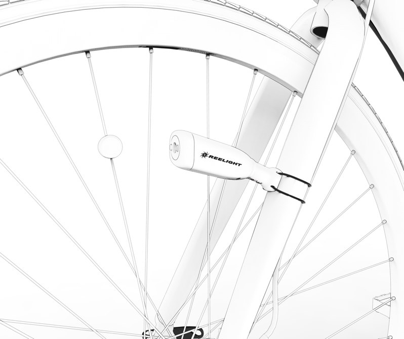
The Reelight safety light with a small built-in generator. The circular spoke unit accelerates the rotor in the light’s generator with each pass. The light itself is mounted on the frame with a coated steel wire rope.
The bike light is always on, yet it doesn’t require any batteries to operate. It also does not have a mechanical part connected to the wheel that often produces an irritating sound. To achieve this design goal, we used simulation to create a power generation system that relies on magnetic induction.
Modeling a Power Generation Source with COMSOL Multiphysics®
The classic power platform for our bicycle safety light is a pure induction-based system. To create sufficient power with this technology, the module mounted on the spokes must span more than one spoke. For our new light, we wanted to keep the spoke unit small and installed on a single spoke to give the user maximum flexibility. In order to accomplish this, we chose to use a simple type of synchronous machine.
Inside the light, a permanent magnet rotor is aligned with a laminated core, on which a coil is wound. The rotor is spun into action by the permanent magnet mounted on the spoke, also called the exciter. This transfers the mechanical energy from the bike to the rotor and lights up the LEDs. An exploded view can be seen below, showing the relevant naming conventions for the generator parts of the light.
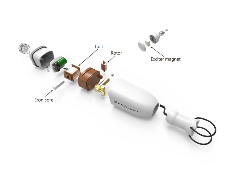
Exploded view of the safety light. The rotor, coil, iron core, and exciter are the subject of further analysis in this blog post.
This concept seems easy to understand, but actually implementing the production is a different story. The bike safety light itself has several design challenges, most of which could be identified by building prototypes and simply playing around with ideas. Since the bike light is a small product, with a limited number of parts, we can use 3D printing to save time and easily test different designs.
When it comes to designing the power generator of the bike light, on the other hand, prototyping has major drawbacks. For instance, the lead time on magnets can stall the iterations on the product. By using the COMSOL Multiphysics® software to model the power generation, we increase the iteration speed in our development cycles. Furthermore, simulation gives us insight into what works, or does not work, in the bike light design. We can use this knowledge to improve the product faster than with only prototyping.
Setting Up the Model in COMSOL Multiphysics®
Even though this power platform is designed for bicycles, it’s still an electrical machine and exhibits some well-known phenomena. Starting the rotor is much like starting an inertia load with a synchronous machine. At some point, depending on the inertia of the rotor and the torque from the magnet, the rotor will be unable to start and the net mechanical transferred power approaches zero.
Since bicycles have a somewhat limited range of operating speeds, it’s possible to find an optimal solution for this range. One of the aims of the model is to investigate the start-up performance of the machine, hence the power generation at different speeds.
The geometry of the machine is simplified to an iron core, rotor with permanent magnets, and the exciter, as depicted below. We use the Rotating Machinery interface and create two identity pairs, each of which has a matching rotation. The exciter rotates proportionally to the speed of the bike, i.e., prescribed rotational velocity, while the rotation of the rotor is calculated with its dynamic equation, i.e., prescribed rotation.
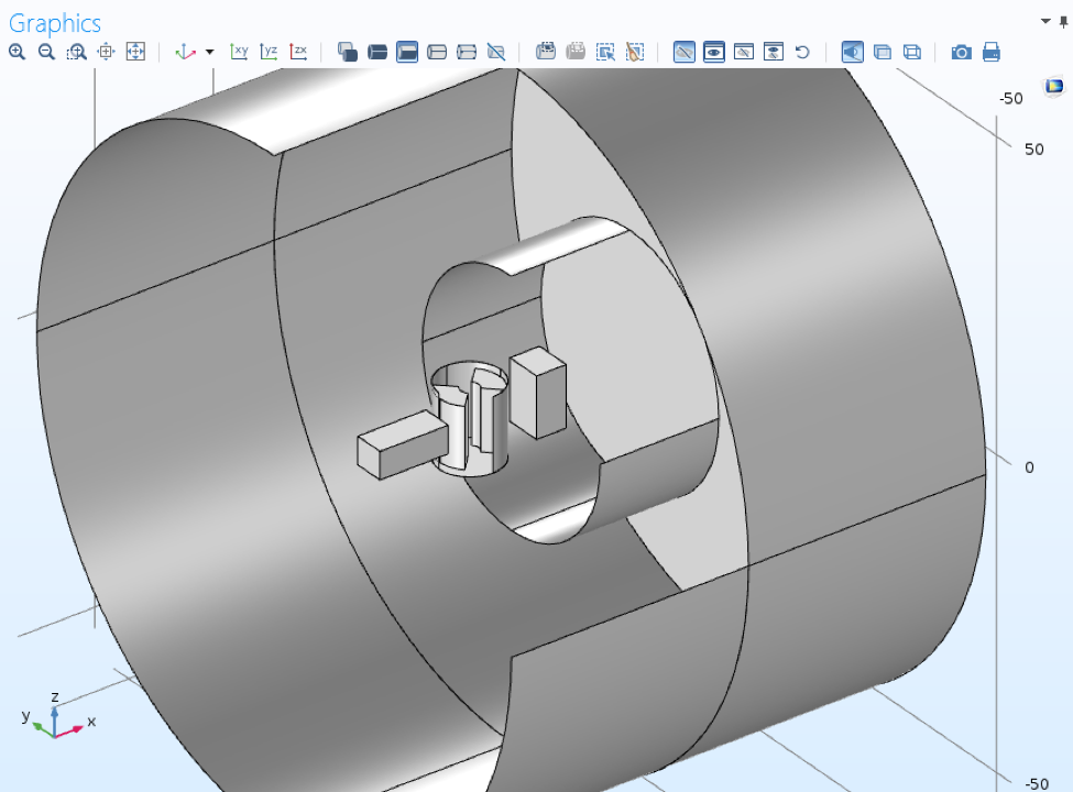
Geometry of the electrical machine, showing the iron core for the coil winding, arc segment permanent magnets, and exciter magnet (the right-most magnet). The remaining geometry is used either for identity pairs in the Rotating Machinery interface or for reasons of mesh control.
To determine the angular velocity and angle of the rotor, per Newton’s second law, we need to know the torque acting on the system and the inertia. We find the inertia of the rotor by setting up an integration for the rotor volume, then using this integration to integrate over the density in the Variables section. An additional 10% is added to the inertia as an experience figure for the shaft, which is not modeled explicitly.

Integration of the rotor’s permanent magnet, used to determine the inertia of the rotor in the Variables section.
We determine the magnetic torque on the rotor by setting up a force calculation, thus accounting for the force between the magnets and the reluctance force. We also add the torque contribution from the damping in the bearing as well as the electrical power. This is set up in the Global Equations node, where the torque summation and the inertia are used to calculate the angle, and angular velocity.
To keep the model simple and save computational power, the induced current is computed by differentiating the flux in the iron core and multiplying it with the number of windings. This approximation of a 3D coil allows us to neglect the coil itself, and its accompanying vector potential formulation, by sacrificing some accuracy. The electrical circuit is implemented in an equation in the Variables section to find the power from the circuit, thus the torque for the rotational equation.
Evaluating the Simulation Results
When running a simulation with moving parts, you can create an animation of the simulation results in COMSOL Multiphysics, as we did for our bike safety light model. The animation seems to fascinate everyone I show it to, most likely because it is easy to visualize and understand the results.
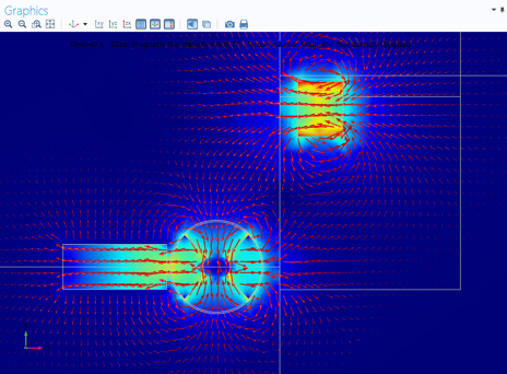
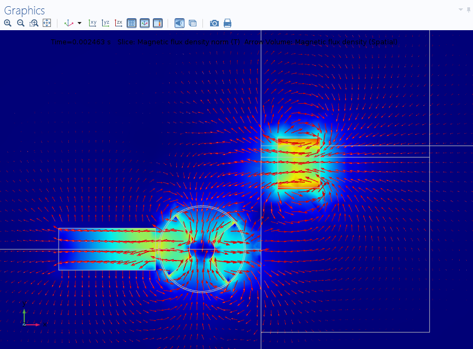
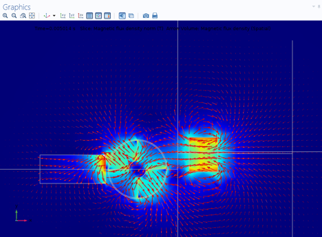
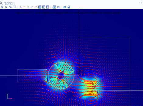
The magnetic field in the coil of the rotor, shown at four different times: t = 0.0 s (top left), t = 0.025 s (top right), t = 0.050 s (bottom left), and t = 0.075 s (bottom right).
The model is sliced through the center of the rotor, perpendicular to the rotational axis. The arrows represent the B vector in the spatial (rotated) frame.
We can also analyze the induced voltage in the coil directly in the model and use this information to estimate the luminous flux from the flash that the light will emit. Several parameters are highly influential on the induced voltage. Since the purpose of the generator is to induce voltage, this parameter is subject to optimization. The voltage output from the coil for this geometry is shown below.
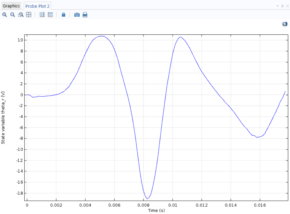
Induced voltage in the stator coil of the rotor.
The torque contributions are the most interesting parameters that this model shows. This is where we can analyze the start-up behavior. In general, the transferred mechanical power is the prerequisite for generating electrical power and more light for our cyclist.
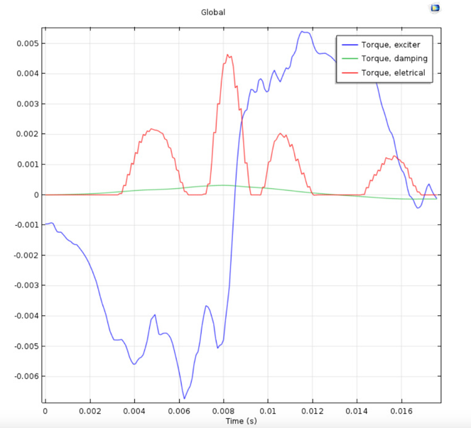
Torque contributions from the exciter, bearing damping, and electrical circuit.
This dynamic model takes approximately 30 minutes to solve and is supported by a series of static sweep studies, where the geometry of the different components can be investigated further and faster. Using simulation, we were able to investigate magnetic induction and optimize a power generation source for our bicycle safety light design.
More Resources on Simulation-Based Design
- Find out about rotating machinery design using the COMSOL Multiphysics® software:
- See how organizations are using simulation-led design in their research
- Browse electromagnetics simulation topics and tutorials on the COMSOL Blog
- Learn more about simulating bicycles and their components:
About the Guest Author
Rune Ryberg Thygesen is a mechanical engineer with a master’s degree in electromechanical system design from Aalborg University. He is a research and development manager at Reelight ApS, a Danish firm that designs battery-free bike lights for the aftermarket.


Comments (0)