
Debugging the Sceptre using JTAG [100810]
Debugging the Sceptre using JTAG, with the help of OpenOCD, GDB, Insight and Eclipse for Windows.
Developing a short program for a microcontroller board can be done using very simple means, but when the software starts to get a bit bigger, these simple means very soon start becoming a limitation, or even bring you to a grinding halt. Elektor’s Sceptre has 512 KB of program memory, and to take full advantage of this, you need appropriate tools, such as a debugger worthy of the name and a tool that loads the executable into the board memory quickly. Buying commercial tools for several thousand pounds is only for the professionals, for whom the time saved is worth more than the cost of the programming tools; so amateurs will have to get by some other way. Fortunately, there are some solutions available.
This is article is part of a large project published in 2010 & 2011 covering several articles:
In the case of the Sceptre and the other members of the large family of boards using ARM processors (and not only ARM), the solution is called JTAG. ARM has specified a JTAG interface using a 20-pin (2×10) connector, which has become fairly standard since a large number of board manufacturers have adopted it. Elektor has done the same and has included it on the InterSceptre and the Automatic Running-in Bench. This interface makes it possible to debug not only the hardware, but also the software and flash memory programming.
We’re not going to talk here about hardware debugging, but confine ourselves to a single component on the JTAG bus: the microcontroller. Even though in the first instance this article addresses the Sceptre, and hence an NXP LPC2148 microcontroller with an ARM7TDMI-S core, the techniques described are just as valid for other controllers. In most cases, all that is needed is to adapt some of the configuration files.
The tools we’re going to be using are GDB and OpenOCD. The former is the GNU Project Debugger open-source debugger, the latter is also an open-source debugger, OCD stands for On-Chip Debugger, but works at a lower level. However, for debugging software for the Sceptre we need to use both of them. Once we’ve taken care of our first steps (that’s what debuggers call them), we’ll add a layer to improve convenience with a graphical interface. But before we get to that point, we’re going to have to start at the bottom of the ladder: the Command prompt.
It may seem odd to split a debugger into a server and a client running on the same computer, but this split has been done for practical reasons. In practice, if the software to be debugged and the debugger are run on the same computer, there is always the risk that a bug in the former may crash the whole system. The debugging information obtained is then lost, along with any other unsaved data, and it will be necessary to restart the computer each time, which ends up getting tiresome. By separating the two, a crash in the system to be debugged is much less troublesome. In our case, this architecture would make it possible to run the GDB server directly on the microcontroller board, but we’re not going to do this (yet), as our software to be embedded (still) hasn’t been developed out enough. At any rate, if the board crashes, this will not crash the computer, so we can run the server and client on the same machine with no danger.
A version of GDB for Windows is included in programming tool chains for ARM like WinARM, for example (see the article about the Sceptre) and Yagarto. For OpenOCD by Dominic Rath, it’s a bit more complicated, because, as the original version used libraries from FTDI without a GPL licence, it is no longer included within Yagarto. WinARM still offers an old version, but a certain Freddi Chopin has had the initiative to produce a version 100 % under a GPL licence for Windows. So download and install OpenOCD 0.4.0 (the latest version) by Freddi Chopin and kick off!
The speed of the probe is important for the speed of debugging. There are a lot of bits to be moved around for each JTAG operation, and each debugging requires several JTAG operations. The is an appreciable difference between a probe on the parallel port capable of producing a JTAG clock at 5 kHz and a USB probe that achieves 6 MHz.
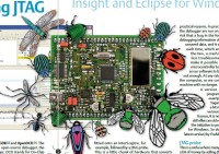
We tried three probes: a basic Wiggler-compatible one on the parallel port, the popular ARM-USB-OCD USB probe from Olimex, and the J-Link Edu from Segger, which is a version of its professional probes cut down for non-commercial use. The Wiggler is easy enough to build yourself (Figures 2 & 3 below), but it’s very slow (the test program is loaded at 957 bits/s, compared to 19 KB/s using the Olimex probe; running a simple line of code in C takes around 3 s). To make this probe work, your computer’s parallel port must be in EPP mode.
The J-Link Edu from Segger is driven by its own GDB server, which is not entirely compatible with OpenOCD, and certain commands are different. OpenOCD does support a J-Link interface, but unfortunately we didn’t manage to make it work with the J-Link Edu. Since the aim of this article is to explain how to debug using only open-source software, we didn’t investigate the J-Link Edu option any further.
In what follows, we’re going to be using the ARM-USB-OCD from Olimex as our JTAG probe.
Connect your JTAG probe to the computer and the microcontroller board, open a Command prompt, and run OpenOCD like this:
Open a second Command prompt and execute:
Before being able to load the executable into the controller, the latter must be halted. GDB can’t stop the processor, but OpenOCD can do it. The monitor command makes it possible to execute an OpenOCD command from GDB:
The file to be used is in the ELF format (not HEX or BIN), as GDB is going to need additional information. For effective debugging, the program must be compiled with a debugging option, which adds information into the executable that is needed for convenient debugging, like the names of the variables and functions. If you examine the makefile, you’ll find for the GCC C compiler the option –gdwarf-2, which indicates that the compiler will include debugging information in the Dwarf 2 format in the executable. It’s thanks to this information that the step command (for example) is able to display the source code corresponding to the point you’re at in the program.
Now, execute the step command a few times, like this:
At the outset, you’ll find yourself right at the start of the program, the part that’s usually written in assembler that initializes the microcontroller. To jump to the main without getting lost in the memory initialization and other loops, insert a breakpoint at the start of the main then let the processor run:
In principle, we ought to always do what we’ve just done at the start of a debugging session. Rather than retype the same commands each time you launch GDB, we can insert them in a commands file (a script) that GDB will execute automatically. By default, GDB looks to see if there isn’t a file named .gdbinit (note this well) somewhere around. If this is the case, it opens it and executes the commands contained in the file. We can also specify a file with another name, thanks to the option ‑command, like this:
Now we’re at the start of our program, the debugging proper can start. This is the moment to position some breakpoints, to inspect the variables, registers, memory, or the stack. Unfortunately, the number of hardware breakpoints, i.e. those that are handled by the hardware itself, is limited. The Sceptre’s microcontroller, the LPC2148, offers only two hardware breakpoints, which is not really very many. That’s why it’s worth debugging a program in RAM, which makes it possible to use software breakpoints handled by GDB and not by the hardware. The number of software breakpoints is in theory unlimited.
When the program is too large to be run from the RAM (the Sceptre’s microcontroller has only 32 kB, to be shared between the program and the data), it has to be loaded into the flash memory and we can’t then use software breakpoints. Certain JTAG probes in this case do allow ‘hardware’ breakpoints to be added. The J-Link Edu from Segger, for example, offers an unlimited number of hardware breakpoints.
The commands used most in a debugging session are probably step, next, finish, continue, break, delete, list and print. A list of these commands, with a short description, is given in Table 1. This table is not exhaustive, practically every command can take several parameters, and still other commands are not included in this list. You’ll be able to find several sites on the Internet offering the missing details relating to GDB. Do note however that there are several versions of GDB, which are not necessarily 100 % compatible. Some use a slightly different syntax and others do not have all the commands. So don’t be surprised if the explanations on a website don’t work with your particular GDB — don’t be afraid to research a bit further. Be aware too that certain GDB commands and functions won’t work with your hardware, quite simply because it doesn’t happen to support them.
Before launching yourself into using a graphical interface, it’s worth familiarizing yourself a little with the commands in text mode and using the GDB console. Try, for example, to understand the difference between step and next, examine the registers, take a look at the stack, etc.
Insight is a free, open source Linux application supported by Red Hat. It’s difficult to compile under and for Windows, and what’s more, it’s quite hard to find an Insight executable pre-compiled for Windows. Reason enough for us to abandon this route and trying something else. So, why go on anyway? Because once you master Insight, it doesn’t work badly at all. It’s a tool that makes for convenient debugging, without useless or cumbersome options.
In fact, an Insight executable for Windows is included in WinARM, the tool chain we’ve chosen for the Sceptre. Certain distributions of Yagarto include it too, but apparently not the most recent distribution.
Unlike Eclipse, Insight incorporates GDB, so when you already have Insight, there’s no point installing GDB as well. In some ways, the tool is a graphical GDB and when you run it, it reads the same initialization script (.gdbinit) as GDB. If this script is correct (Insight is a bit quirky and you have to obey the correct order for certain commands), the debugger launches and shows the source code highlighted on the line where the program stopped (if a breakpoint has been set in advance, naturally). Note that it’s imperative to launch OpenOCD as previously described before starting Insight.
From the main window (Source Window, Figure 6 below), we have access to additional windows for displaying the local variables, registers, stack, memory, breakpoints, and the GDB console. As you move around within your program, all these windows are updated by the software, with the latest changes highlighted. It’s a bit more convenient that typing print commands after each step.
For the GUI to be able to update everything that’s displayed, it takes a lot of extra JTAG transactions each time a command is executed. If your JTAG probe is slow, this can take some time, whence the interest of getting yourself a suitable probe.
Insight’s GDB console lets you do the same thing as the GDB console described earlier, except that the results are displayed in other windows. Access to the GDB console is very handy when you lose control of the debugging and Insight has to execute commands it doesn’t know (for example, monitor reset).
It sometimes happens that an operation leads to loss of the connection between GDB and OpenOCD without your realizing — for example, if you load a new file to debug. So do keep an eye on the OpenOCD window to check that the connection is still in place.
Once Eclipse/CDT is installed, run it and choose a location for the workspace, the place where Eclipse will go and store the project(s). Since we already have the source code for our application, we’re going to import everything. For speed, use File -> New -> Makefile Project with Existing Code. Then browse your way to your existing project (Existing Code Location) and change the name of the project (Project Name) if necessary. Select <none> as Toolchains for Indexer Settings and check the programming language(s) used. Press the Finish button, and you’re there.
Eclipse offers all sorts of views of a project, called Perspectives. By default, it opens the Resource view, but we want the C/C++ view (Window -> Open Perspective -> Other…). You can close the Resource view to eliminate one button.
In order to test your project and at the same time the installation of Eclipse, you can try a make clean (Project -> Clean…), followed by a make all (Project -> Build Project). Eclipse/CDT presumes that the compilation and GDB tools are present somewhere on your computer. You can indicate the path to GDB, but make has to be able to locate it via the ‘global’ path in Windows. If you use several different compilation chains (WinARM, Yagarto, or others), the simplest thing is to use an adapted makefile for each tool chain.
If these two tests were successful, you can move on to debugging.
As before, you must run OpenOCD before starting the debugging. It is possible to configure an external tool (Run -> External Tools -> External Tools Configurations…) for this purpose, which will let you launch OpenOCD from Eclipse; but just using the Command prompt works too.
Open the Debug perspective. The debugger has to be configured before use. You can access debugger configuration via the menu Run -> Debug Configurations or via the small arrow to the right of the Debug button (with the little beetle). Select GDB Hardware Debugging and click the button New (the blank page with a small ‘+’). There are three tabs to indicate : Main, Debugger and Startup. Refer to Figures 8, 9, and 10 (below) to find out how to configure your debugger. Those parameters not seen in these figures have kept their default values. Note that the Startup tab contains a window where you can enter the commands to be executed when GDB starts up. These are the same commands as those used above and that we have put in our .gdbinit file.
Launch the debugger. If this is the first time for the current project, Eclipse won’t offer it at the outset and you’ll have to start by configuring the debugger by pressing the Debug button. The next time, Eclipse will propose the project when you press the button with the beetle. As soon as Eclipse is correctly configured, you get a debugging view like the one in Figure 11 below. Get yourself a big screen, as Eclipse offer lots of windows and you’ll need the room to display them all. At the bottom left of this figure, you can see the GDB console where you type in yourself the GDB commands (Eclipse has disabled the (gdb) prompt). Don’t let yourself be distracted by all the buttons, icons, and tabs that decorate the windows, concentrate first of all on their contents.
You can move around in your program using the F5, F6, and F7 keys and the options offered in the Run menu. If you want additional windows, go to Window -> Show View.
For this to work, you need to configure OpenOCD, for example with the help of OpenOCD’s target configuration file, like this:
From GDB, we now launch the command:
Table 1. The most-used GDB commands with a short description. Most of the commands accept any sort of parameters. Consult the help or the Internet for further details.
This is article is part of a large project published in 2010 & 2011 covering several articles:
- The Sceptre - hardware (main article)
- The Sceptre - software
- Debugging the Sceptre over JTAG (this article)
- The InterSceptre - I/O expansion board
- The Sceptre meets Arduino
- The Sceptre meets Oberon
- Graphic display shield for the Sceptre
In the case of the Sceptre and the other members of the large family of boards using ARM processors (and not only ARM), the solution is called JTAG. ARM has specified a JTAG interface using a 20-pin (2×10) connector, which has become fairly standard since a large number of board manufacturers have adopted it. Elektor has done the same and has included it on the InterSceptre and the Automatic Running-in Bench. This interface makes it possible to debug not only the hardware, but also the software and flash memory programming.
We’re not going to talk here about hardware debugging, but confine ourselves to a single component on the JTAG bus: the microcontroller. Even though in the first instance this article addresses the Sceptre, and hence an NXP LPC2148 microcontroller with an ARM7TDMI-S core, the techniques described are just as valid for other controllers. In most cases, all that is needed is to adapt some of the configuration files.
The tools we’re going to be using are GDB and OpenOCD. The former is the GNU Project Debugger open-source debugger, the latter is also an open-source debugger, OCD stands for On-Chip Debugger, but works at a lower level. However, for debugging software for the Sceptre we need to use both of them. Once we’ve taken care of our first steps (that’s what debuggers call them), we’ll add a layer to improve convenience with a graphical interface. But before we get to that point, we’re going to have to start at the bottom of the ladder: the Command prompt.
OpenOCD and GDB
Setting up a debugging environment based on GDB and OpenOCD may seem a bit off-putting at first sight (and even at the second), which is why we’re going about it gently. Figure 1 (below) shows the block diagram of the environment we’re going to be setting up. Right over on the left, we have a microcontroller board, a Sceptre fitted onto an InterSceptre, for example, followed by a JTAG probe. This is a little chunk of hardware that converts the JTAG bus into a USB or parallel port (or even some other type) so as to be able to connect up to a computer. The JTAG probe is driven by a GDB server, a piece of software able to convert high-level debugging commands into low-level JTAG operations. OpenOCD is going to be acting as our GDB server. The GDB client, the GDB software itself, sends debugging requests to the server and processes the replies received. And lastly, a graphical interface completes the environment. This will save you a lot of work by looking after sending the large number of commands needed for debugging a piece of software, and will present the results in a practical, convenient manner.It may seem odd to split a debugger into a server and a client running on the same computer, but this split has been done for practical reasons. In practice, if the software to be debugged and the debugger are run on the same computer, there is always the risk that a bug in the former may crash the whole system. The debugging information obtained is then lost, along with any other unsaved data, and it will be necessary to restart the computer each time, which ends up getting tiresome. By separating the two, a crash in the system to be debugged is much less troublesome. In our case, this architecture would make it possible to run the GDB server directly on the microcontroller board, but we’re not going to do this (yet), as our software to be embedded (still) hasn’t been developed out enough. At any rate, if the board crashes, this will not crash the computer, so we can run the server and client on the same machine with no danger.
A version of GDB for Windows is included in programming tool chains for ARM like WinARM, for example (see the article about the Sceptre) and Yagarto. For OpenOCD by Dominic Rath, it’s a bit more complicated, because, as the original version used libraries from FTDI without a GPL licence, it is no longer included within Yagarto. WinARM still offers an old version, but a certain Freddi Chopin has had the initiative to produce a version 100 % under a GPL licence for Windows. So download and install OpenOCD 0.4.0 (the latest version) by Freddi Chopin and kick off!
JTAG probe
This is a niche where many electronics merchants are trying to make a bit of money by selling JTAG probes that are more or less powerful. Broadly speaking, the differences between all these probes lie in the maximum speed of communication on the JTAG bus (the faster it is, the more convenient the debugging) and in their ability to program the microcontroller or not. Before you go out and order a probe with all the bells and whistles, be aware that OpenOCD is perfectly capable of programming a large number of controllers and flash memories, including those of the Sceptre, at a perfectly acceptable speed (depending on the probe). The programming option is of particular interest to a production unit that has to program a large number of chips.The speed of the probe is important for the speed of debugging. There are a lot of bits to be moved around for each JTAG operation, and each debugging requires several JTAG operations. The is an appreciable difference between a probe on the parallel port capable of producing a JTAG clock at 5 kHz and a USB probe that achieves 6 MHz.
We tried three probes: a basic Wiggler-compatible one on the parallel port, the popular ARM-USB-OCD USB probe from Olimex, and the J-Link Edu from Segger, which is a version of its professional probes cut down for non-commercial use. The Wiggler is easy enough to build yourself (Figures 2 & 3 below), but it’s very slow (the test program is loaded at 957 bits/s, compared to 19 KB/s using the Olimex probe; running a simple line of code in C takes around 3 s). To make this probe work, your computer’s parallel port must be in EPP mode.
The J-Link Edu from Segger is driven by its own GDB server, which is not entirely compatible with OpenOCD, and certain commands are different. OpenOCD does support a J-Link interface, but unfortunately we didn’t manage to make it work with the J-Link Edu. Since the aim of this article is to explain how to debug using only open-source software, we didn’t investigate the J-Link Edu option any further.
In what follows, we’re going to be using the ARM-USB-OCD from Olimex as our JTAG probe.
Debugging in text mode
Check first that Windows (or you yourself) can find OpenOCD and GDB.Connect your JTAG probe to the computer and the microcontroller board, open a Command prompt, and run OpenOCD like this:
openocd -f interface/olimex-arm-usb-ocd.cfg -f board/elektor_sceptre.cfg
The CFG files specified depend on your hardware. We’re using the ARM-USB-OCD probe from Olimex with a Sceptre board fitted to an InterSceptre board.Open a second Command prompt and execute:
arm-none-eabi-gdb
Next, we need to execute a series of commands to connect GDB to OpenOCD and to load the executable in the controller’s RAM memory (when debugging a program in RAM). The commands must be entered in GDB (indicated by the (gdb) prompt):
(gdb) target remote localhost:3333
This rather strange command pretends that we’re going to debug our target remotely (remote), although it is actually connected to our computer (localhost). If OpenOCD is listening on port 3333 (the default value), you should see appear in the OpenOCD window an Info message saying accepting ’gdb’ connection from 0 (Figure 4). GDB and OpenOCD will now be able to communicate.Before being able to load the executable into the controller, the latter must be halted. GDB can’t stop the processor, but OpenOCD can do it. The monitor command makes it possible to execute an OpenOCD command from GDB:
(gdb) monitor reset halt
If this command, intended to perform a reset followed by a halt, has worked properly, the microcontroller is now stopped. Before continuing, check that GDB and OpenOCD are displaying the message target state: halted. If this is the case, we can load the executable file into GDB and into the microcontroller (if necessary):
(gdb) file test_ram.elf
(gdb) load
The first command reads the file and the second loads it into the microcontroller’s RAM memory. Note that you must not execute the load command if the program is already loaded into flash memory. We found we were unable to successfully debug a program in RAM while another was already loaded in flash.The file to be used is in the ELF format (not HEX or BIN), as GDB is going to need additional information. For effective debugging, the program must be compiled with a debugging option, which adds information into the executable that is needed for convenient debugging, like the names of the variables and functions. If you examine the makefile, you’ll find for the GCC C compiler the option –gdwarf-2, which indicates that the compiler will include debugging information in the Dwarf 2 format in the executable. It’s thanks to this information that the step command (for example) is able to display the source code corresponding to the point you’re at in the program.
Now, execute the step command a few times, like this:
(gdb) step
When you want to repeat the previous command, all you have to do is press Enter. After each step, GDB displays the line of the file carrying the next instruction that the microcontroller must execute, along with the current line itself (with comments, if there are any).At the outset, you’ll find yourself right at the start of the program, the part that’s usually written in assembler that initializes the microcontroller. To jump to the main without getting lost in the memory initialization and other loops, insert a breakpoint at the start of the main then let the processor run:
(gdb) break main
(gdb) continue
A little later on, GDB issues a message along the lines of:
Breakpoint 1, main () at src/main.c:73
and there you are in your code (Figure 5, below).In principle, we ought to always do what we’ve just done at the start of a debugging session. Rather than retype the same commands each time you launch GDB, we can insert them in a commands file (a script) that GDB will execute automatically. By default, GDB looks to see if there isn’t a file named .gdbinit (note this well) somewhere around. If this is the case, it opens it and executes the commands contained in the file. We can also specify a file with another name, thanks to the option ‑command, like this:
arm-none-eabi-gdb -command gdb_cmd.txt
Be aware that the use of a script file can sometimes lead to difficulties — perhaps because the commands are sent too fast one after the other? If this happens, you need to interrupt GDB using <ctrl><c>, stop the microcontroller (monitor reset halt) and, in the case of a program in RAM, reload the program using load.Now we’re at the start of our program, the debugging proper can start. This is the moment to position some breakpoints, to inspect the variables, registers, memory, or the stack. Unfortunately, the number of hardware breakpoints, i.e. those that are handled by the hardware itself, is limited. The Sceptre’s microcontroller, the LPC2148, offers only two hardware breakpoints, which is not really very many. That’s why it’s worth debugging a program in RAM, which makes it possible to use software breakpoints handled by GDB and not by the hardware. The number of software breakpoints is in theory unlimited.
When the program is too large to be run from the RAM (the Sceptre’s microcontroller has only 32 kB, to be shared between the program and the data), it has to be loaded into the flash memory and we can’t then use software breakpoints. Certain JTAG probes in this case do allow ‘hardware’ breakpoints to be added. The J-Link Edu from Segger, for example, offers an unlimited number of hardware breakpoints.
The commands used most in a debugging session are probably step, next, finish, continue, break, delete, list and print. A list of these commands, with a short description, is given in Table 1. This table is not exhaustive, practically every command can take several parameters, and still other commands are not included in this list. You’ll be able to find several sites on the Internet offering the missing details relating to GDB. Do note however that there are several versions of GDB, which are not necessarily 100 % compatible. Some use a slightly different syntax and others do not have all the commands. So don’t be surprised if the explanations on a website don’t work with your particular GDB — don’t be afraid to research a bit further. Be aware too that certain GDB commands and functions won’t work with your hardware, quite simply because it doesn’t happen to support them.
Before launching yourself into using a graphical interface, it’s worth familiarizing yourself a little with the commands in text mode and using the GDB console. Try, for example, to understand the difference between step and next, examine the registers, take a look at the stack, etc.
Adding a graphical interface
Even though debugging in text mode is very powerful and instructive, typing in all the commands manually soon gets tiresome. So to make the debugger’s life a bit easier, several graphical interfaces have been developed for GDB. One graphical interface (GUI, from Graphical User Interface) lets you see the source code without executing the list command, and keeps the variable, register, and stack values automatically updated; it displays the breakpoints clearly, along with the point you’re at in the program. Several GUIs exist, but not all of them are suitable for debugging a microcontroller board. The two GUIs most used for this purpose are Eclipse and Insight. Eclipse is a powerful, sophisticated, free, integrated multi-platform environment. By adding a plug-in, it also be used as a GUI for GDB. But setting up an Eclipse environment for GDB is a bit complicated, so we’re going to start by taking a look at Insight, a GUI born and bred for GDB.Insight is a free, open source Linux application supported by Red Hat. It’s difficult to compile under and for Windows, and what’s more, it’s quite hard to find an Insight executable pre-compiled for Windows. Reason enough for us to abandon this route and trying something else. So, why go on anyway? Because once you master Insight, it doesn’t work badly at all. It’s a tool that makes for convenient debugging, without useless or cumbersome options.
In fact, an Insight executable for Windows is included in WinARM, the tool chain we’ve chosen for the Sceptre. Certain distributions of Yagarto include it too, but apparently not the most recent distribution.
Unlike Eclipse, Insight incorporates GDB, so when you already have Insight, there’s no point installing GDB as well. In some ways, the tool is a graphical GDB and when you run it, it reads the same initialization script (.gdbinit) as GDB. If this script is correct (Insight is a bit quirky and you have to obey the correct order for certain commands), the debugger launches and shows the source code highlighted on the line where the program stopped (if a breakpoint has been set in advance, naturally). Note that it’s imperative to launch OpenOCD as previously described before starting Insight.
From the main window (Source Window, Figure 6 below), we have access to additional windows for displaying the local variables, registers, stack, memory, breakpoints, and the GDB console. As you move around within your program, all these windows are updated by the software, with the latest changes highlighted. It’s a bit more convenient that typing print commands after each step.
For the GUI to be able to update everything that’s displayed, it takes a lot of extra JTAG transactions each time a command is executed. If your JTAG probe is slow, this can take some time, whence the interest of getting yourself a suitable probe.
Insight’s GDB console lets you do the same thing as the GDB console described earlier, except that the results are displayed in other windows. Access to the GDB console is very handy when you lose control of the debugging and Insight has to execute commands it doesn’t know (for example, monitor reset).
It sometimes happens that an operation leads to loss of the connection between GDB and OpenOCD without your realizing — for example, if you load a new file to debug. So do keep an eye on the OpenOCD window to check that the connection is still in place.
Let’s end this section with a few general comments.
- On our test computer, launching the copy of Insight included in WinARM produces a warning Unknown ARM EABI version 0x5000000. Ignoring this warning doesn’t seem to stop the tool working properly. If you know where to find a more recent version of Insight pre-compiled for Windows, please let us know.
- Figure 7 below shows how to configure Insight by hand (File -> Target Settings…).
Better still
Insight is already a very good tool for debugging an application running on a microcontroller board, but there is better yet. Eclipse (see above) is an integrated development environment (IDE) with all mod cons, written in Java, which lets you not only debug an application, but also edit source code, launch compilation, and start other software and tools, all from the same environment. But there’s a price to pay for all this luxury: it’s hard to install an Eclipse environment without consulting several websites, as Eclipse is a generic IDE stuffed with options (often incomprehensible) to satisfy the needs of all comers. So we’re not going to tell you how to go about it here, but direct you to the Yagarto site, for example, where there’s a very detailed tutorial on the subject. Do note that it’s not enough to just install Eclipse, you also need to install the CDT (C/C++ Development Tooling) plug-in that converts Eclipse into an IDE for developing software in C/C++ and adds the debugging function to it.Once Eclipse/CDT is installed, run it and choose a location for the workspace, the place where Eclipse will go and store the project(s). Since we already have the source code for our application, we’re going to import everything. For speed, use File -> New -> Makefile Project with Existing Code. Then browse your way to your existing project (Existing Code Location) and change the name of the project (Project Name) if necessary. Select <none> as Toolchains for Indexer Settings and check the programming language(s) used. Press the Finish button, and you’re there.
Eclipse offers all sorts of views of a project, called Perspectives. By default, it opens the Resource view, but we want the C/C++ view (Window -> Open Perspective -> Other…). You can close the Resource view to eliminate one button.
In order to test your project and at the same time the installation of Eclipse, you can try a make clean (Project -> Clean…), followed by a make all (Project -> Build Project). Eclipse/CDT presumes that the compilation and GDB tools are present somewhere on your computer. You can indicate the path to GDB, but make has to be able to locate it via the ‘global’ path in Windows. If you use several different compilation chains (WinARM, Yagarto, or others), the simplest thing is to use an adapted makefile for each tool chain.
If these two tests were successful, you can move on to debugging.
As before, you must run OpenOCD before starting the debugging. It is possible to configure an external tool (Run -> External Tools -> External Tools Configurations…) for this purpose, which will let you launch OpenOCD from Eclipse; but just using the Command prompt works too.
Open the Debug perspective. The debugger has to be configured before use. You can access debugger configuration via the menu Run -> Debug Configurations or via the small arrow to the right of the Debug button (with the little beetle). Select GDB Hardware Debugging and click the button New (the blank page with a small ‘+’). There are three tabs to indicate : Main, Debugger and Startup. Refer to Figures 8, 9, and 10 (below) to find out how to configure your debugger. Those parameters not seen in these figures have kept their default values. Note that the Startup tab contains a window where you can enter the commands to be executed when GDB starts up. These are the same commands as those used above and that we have put in our .gdbinit file.
Launch the debugger. If this is the first time for the current project, Eclipse won’t offer it at the outset and you’ll have to start by configuring the debugger by pressing the Debug button. The next time, Eclipse will propose the project when you press the button with the beetle. As soon as Eclipse is correctly configured, you get a debugging view like the one in Figure 11 below. Get yourself a big screen, as Eclipse offer lots of windows and you’ll need the room to display them all. At the bottom left of this figure, you can see the GDB console where you type in yourself the GDB commands (Eclipse has disabled the (gdb) prompt). Don’t let yourself be distracted by all the buttons, icons, and tabs that decorate the windows, concentrate first of all on their contents.
You can move around in your program using the F5, F6, and F7 keys and the options offered in the Run menu. If you want additional windows, go to Window -> Show View.
As in the section on Insight, we’re going to end here with a few miscellaneous comments.
- If you can’t manage to restart a debugging session, first delete all the breakpoints (Run -> Remove all Breakpoints).
- To load the debugging symbols, Eclipse executes GDB’s command symbol-file instead of the file command. As a result, the executable is not loaded by GDB and a subsequent load command will fail. So in the case of debugging from the RAM, you’ll have to explicitly add the file command to the list of start-up commands (or load the program manually in the GDB console). In that case, remember to specify the full pathname, using double slashes ’//’ in place of each ‘\’, as in Figure 10 below.
Loading a program into flash memory
When you are the lucky owner of a JTAG probe compatible with OpenOCD, there’s nothing to stop you also using it for loading the executable into the processor’s or microcontroller board’s flash memory. Note that the J-Link Edu won’t let you programme the flash memory without an additional licence (unless you can manage to make it work with OpenOCD). Programming by JTAG is especially worthwhile when the application is bulky and the controller’s default programming technique is slow, as is the case for the Sceptre’s LPC2148, which uses a serial link. Thanks to the USB JTAG probe we used for this article, the Sceptre programming time has been reduced by a factor of nearly ten!For this to work, you need to configure OpenOCD, for example with the help of OpenOCD’s target configuration file, like this:
flash bank lpc2148.flash lpc2000 0x0 0x7d00000 lpc2148.cpu lpc2000_v2 12000 calc_checksum
The value 12000 corresponds to the processor’s clock frequency in kHz. The calc_checksum parameter is required to insert a checksum into the executable, which is obligatory for the LPC2148 to be able to run the program. If your executable already has this checksum, you can delete the parameter and you’ll avoid a warning during programming.From GDB, we now launch the command:
(gdb) monitor flash write_image <filename>
where <filename> indicates the full pathname of the executable file (in BIN, ELF, HEX, etc. format, see the OpenOCD manual) in which every ‘\’ has been replaced by a ‘/’.| Command | Description |
| apropos | Lets you search in the help on a keyword. |
| backtrace (bt) | Shows where you are in the program according to the stack. |
| break (b) | Set a breakpoint. E.g. break main |
| clear | Deletes a breakpoint. |
| continue (c) | Continues execution of the program. <ctrl><c> lets you interrupt the program. |
| delete (d) | Deletes one, several, or all breakpoints. |
| finish | Terminates the current subroutine. |
| help (h) | Displays gdb help. help followed by a command name lets you obtain help about that command. E.g. help print |
| info (i) | Displays additional information about something. Must be followed by a parameter, like ‘info sources’ to display a list of the source files used by the program. |
| list (l) | Lets you display a number of lines (default = 10) of the source code. |
| next (n) | Executes the next line without entering a subroutine, i.e. the subroutine call is treated as a simple line of the program. The subroutine is executed. |
| print (p) | Shows the value of a variable or register. |
| quit (q) | Terminates GDB. |
| run (r) | Starts execution of a program from the beginning. |
| set | Lets you enable or disable a GDB option. |
| show | Shows the status of a GDB option. show without any parameters displays all of them. |
| step (s) | Executes the next line. Enter into a subroutine. |
| until | Continues execution until it reaches a certain line or subroutine. until toto is equivalent to break toto ; continue |
| watch | Stops execution of the program when the specified condition becomes true. |
| where | See backtrace. |
| <ctrl><c> | Forces GDB to stop execution of the program. |
| <enter> | Repeats the last command. |
Discussie (0 opmerking(en))